Earned Schedule Explained: Fixing EVM's Time Blind Spot

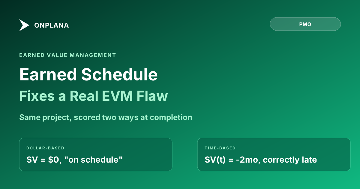
Classic earned value has a schedule score that cannot fail. Run the numbers on the day a project finally closes out two months late, and schedule variance reads $0 and SPI reads 1.00, the identical score a project finishing exactly on time would post. That is not a rounding artifact. It is the dollar-based formula working exactly as designed, which is the entire problem: earned schedule fixes it by measuring the same schedule gap in time instead of dollars, so a late project keeps reporting late, even after it closes.

The direct answer: Earned schedule (ES) restates a project's schedule performance in units of time rather than currency. Instead of comparing Earned Value to Planned Value in dollars, it finds the point on the planned value curve where today's EV should have occurred, and calls that point ES. Schedule variance in time, SV(t) = ES minus actual time elapsed, does not collapse to zero at completion the way dollar-based schedule variance always does. Walt Lipke introduced the method in a 2003 paper, "Schedule is Different," for The Measurable News, and the flaw it fixes is well documented: at project completion, dollar-based SV is always 0 and SPI is always 1.0, whatever the actual finish date turns out to be.

Why Dollar-Based Schedule Variance Breaks Down

Classic EVM's schedule variance is SV = EV minus PV, and its schedule performance index is SPI = EV / PV, both priced in the same currency as the budget. That works fine mid-project, but it has a structural flaw baked into the math: at completion, Earned Value always equals the total approved budget (100 percent of the work is done, so EV = BAC), and Planned Value has already flattened out at BAC too, because the planned value curve cannot rise past the total budget once the project passes its planned finish date. EV minus PV at that point is BAC minus BAC, which is always zero, regardless of whether the project finished on the original date or eighteen months late. SPI has the same problem: EV / PV converges to BAC / BAC, which is always 1.0.

This is not a hypothetical edge case. It is the reason a program running six months behind schedule can show a perfectly healthy SPI in its final status report, and it is exactly the gap earned schedule was built to close.

What Earned Schedule Actually Calculates

Earned schedule finds the moment on the planned value curve where the project's current earned value should have occurred, then measures against that moment instead of against dollars.

ES = C + (EV − PV_C) / (PV_C+1 − PV_C)

Where C is the last complete period in which cumulative planned value was still at or below the current earned value. The fraction interpolates the fractional period between C and C+1, assuming the planned value curve grows roughly linearly within that one period.

Two time-based figures follow directly from ES:

• SV(t) = ES − AT (actual time elapsed). Negative means behind schedule, in time units.
• SPI(t) = ES / AT. Below 1.0 means behind; above 1.0 means ahead.
• IEAC(t) = PD / SPI(t), an independent forecast of total project duration, where PD is the originally planned duration.

Schedule Variance vs Earned Schedule, Side by Side

	Dollar-based (SV, SPI)	Time-based (SV(t), SPI(t))
Unit	Currency	Time (months, weeks, days)
Formula	SV = EV − PV; SPI = EV / PV	SV(t) = ES − AT; SPI(t) = ES / AT
Behavior at completion	Always 0 / always 1.0	Reflects the true time gap
Signals a late finish after the fact	No	Yes
Extra input required	None beyond standard EVM	None; only an interpolation step on data already collected
Forecast produced	EAC (cost)	IEAC(t) (duration)
Best paired with	Cost control	Critical path analysis

A Worked Comparison

Take a $1,200,000 project baselined to finish in 12 months. By month 10, the plan expects $960,000 of cumulative value earned; by month 11, $1,080,000. The project has actually earned $900,000 by month 10, ten months of actual time elapsed.

Dollar-based: SV = $900,000 − $960,000 = −$60,000. SPI = 900,000 / 960,000 = 0.94. Mildly behind.

Time-based: ES interpolates between month 9 ($860,000 planned) and month 10 ($960,000 planned): ES = 9 + (900,000 − 860,000) / (960,000 − 860,000) = 9.4. SV(t) = 9.4 − 10 = −0.6 months. SPI(t) = 9.4 / 10 = 0.94. At month 10, the two methods agree: both say the project is running about six percent behind.

Now fast-forward to actual completion at month 14, two months late. Earned Value has reached the full $1,200,000 budget, and so has Planned Value (it flattened at the budget once the plan's 12-month finish passed). Dollar-based: SV = $1,200,000 − $1,200,000 = $0. SPI = 1.00. Time-based: ES = 12 (the point on the planned value curve where $1,200,000 was scheduled to be earned). SV(t) = 12 − 14 = −2 months. SPI(t) = 12 / 14 ≈ 0.86.

Both scorecards are computed from the same underlying data, on the same closing day. Only the units differ, and only one of them tells the truth once the project is done.

When the Difference Actually Becomes Decision-Relevant

Early in a project, dollar-based SPI and time-based SPI(t) usually agree, as the worked example above shows at month 10: both read 0.94. The gap opens specifically as a project nears its planned finish date, because that is exactly when the planned value curve flattens out at the budget and starts dragging dollar-based SPI toward the false comfort of 1.0. The closer a status report sits to the planned finish line, the less a dollar-based SPI reading should be trusted at face value, and the more it is worth checking SPI(t) or reading variance against the baseline directly instead.

That timing has a practical consequence for reporting cadence: a PMO that only pulls out earned schedule once a month is behind never gets the early warning. Track SPI(t) alongside SPI every period from the start, the same way SPI and CPI need reading together and not separately, so the divergence between the two schedule numbers is visible well before the project reaches the zone where dollar-based SV stops being useful at all.

Earned Schedule Still Needs a Real Baseline

Every figure above assumes the planned value curve comes from a baseline that actually represents an executable schedule. If the underlying network has dangling dependencies or unresolved constraint conflicts, the PV curve it produces looks smooth on a chart and is arithmetically meaningless, the same baseline problem that undermines earned value management generally. Run the free Schedule Health Check against the .mpp or MSPDI export before baselining a schedule for either EVM or earned schedule reporting; it flags the dangling tasks and constraint conflicts that would otherwise quietly corrupt every PV, ES, and SV(t) number calculated against that baseline for the rest of the project. This post sits alongside the rest of the schedule and cost controls library, from critical path math to baseline drift reading.

Check your baseline before you trust the schedule numbers Upload an .mpp or MSPDI XML to the free Schedule Health Check and get a structural audit: dangling tasks, broken dependencies, and constraint conflicts that would otherwise distort every PV-based calculation downstream. No signup required. → Run the Schedule Health Check